Smooth-As-Butter Robot Policies
Introduction
Lately at Cobot, we’ve been investigating various Vision-Language-Action models (VLAs), and have found a need to have smooth reactive policy rollouts while still maintaining the raw power of these heavy models. Real-Time Action Chunking (RTC) is one recent answer to combining these two aspects (slow inference while maintaining smoothness and reactivity). When we tried it ourselves, we noticed small but perceptible discontinuities between chunks, and found there still seemed to be room for improvement. In this article, we’ll share a tweak we made to their algorithm to get smooth-as-butter robot policies.
To kick this blog post off, here’s a video (1x speed) of a fine-tuned π₀ policy using RTC and our preferred settings.
Edit (Dec 21, 2025) - A follow-up talk to this article is now available here on YouTube.
Preliminaries
Ever since Diffusion Policy and ACT, the predominant approach to robot learning has been imitation learning with observations (camera streams, proprioception) as inputs, and sequences (aka “chunks”) of actions (usually positional targets in either joint space or task space) as targets. The key motivator behind predicting action chunks, rather than individual actions, is to match the strong temporal correlation seen in action sequences produced by a human demonstrator.
To put this into more practical terms, one typical setup might involving controlling a pair of ALOHA arms, by commanding joint angles at 50 Hz (or 20 ms between actions).
One challenge with heavier modelling approaches (like VLAs or various flavors of diffusion models) is that inference time might take longer than the control loop time, 20 ms in our example case. For example, we might use a VLA like π₀, to produce chunks of 50 actions (1 second’s worth) at a time, which on an Nvidia 4090 takes about 80~90 ms. A simple, and usually effective, approach is to just roll out a chunk, pause and wait for inference, then roll out the next chunk, and so on. But there are a couple of reasons we might not want this stutter step approach:
- the environment or task might be dynamic, meaning we can’t afford to stop
- if our policy takes in joint velocities, or a history of observations as input, the pauses will be out-of-distribution relative to the training data
- humans working with these robots will mostly prefer to see smooth movements
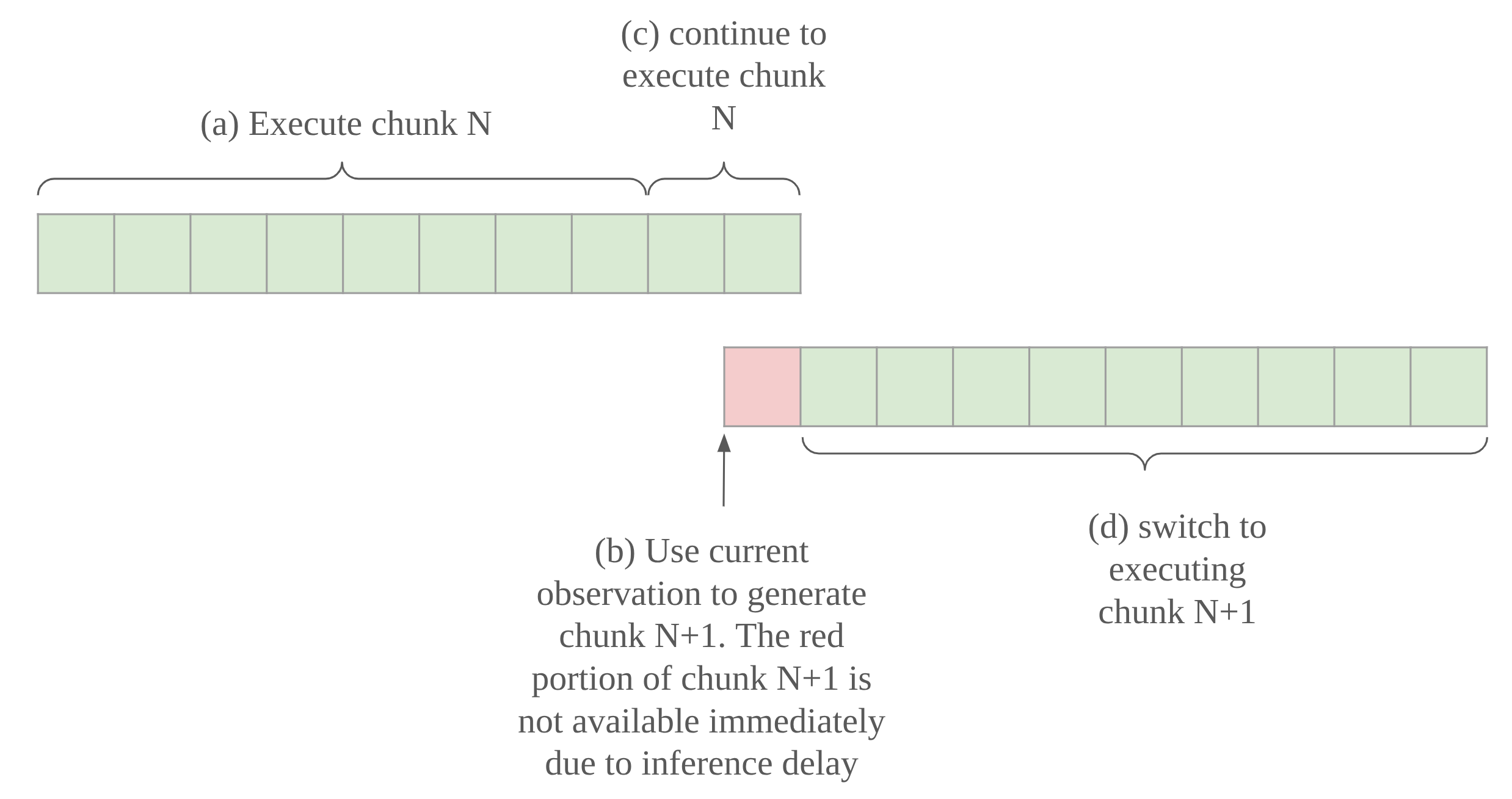
Real-Time Action Chunking (RTC) is one of several recent approaches to dealing with these challenges. The key idea is to “start inference before you need the next action chunk”, and is visualized in the diagram below:
(a) First, let’s assume we have an action chunk to execute. Maybe it’s the first one in our rollout. To help put concrete numbers on it, imagine each cell represents 5 actions or 100 ms.
(b) At some point, knowing that our inference delay is 90 ms, we have to feed the most current observation into our model to get a new action chunk. We know we’ll have the new chunk just on time, because we have over 90 ms left in the current chunk.
(c) So, of course we must continue to execute the current chunk while we wait.
(d) Just as we approach the end of the runway on the current chunk, the model returns the next chunk, so we can switch to executing those actions instead.
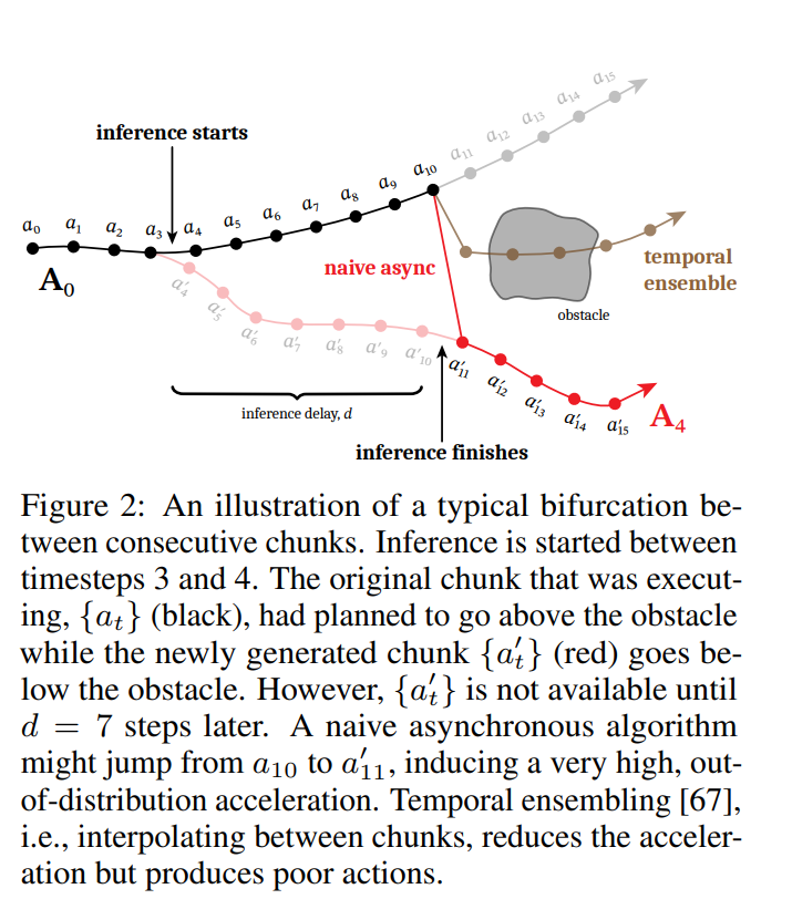
Excellent! But we still have an issue. Often times, the transition from chunk N to chunk N+1 is not going to be smooth. Figure 2 in the RTC paper does a fantastic job of illustrating this problem, so we will not attempt to add any more explanation beyond it.
The second key idea of RTC is to condition the next chunk generation with the prior chunk. Basically, we want to tell our model to produce a chunk whose start is consistent with the end of the prior chunk. Luckily flow modelling (as used in π₀) offers us a toolkit of conditioning methods, one of which is inpainting. That is, rather than generating our new chunk from scratch, we explicitly tell our model that we want the first part of the new chunk to look like the last part of our prior chunk.
- First of all, if you’re familiar with diffusion modeling but not flow matching, don’t worry. They are really two sides of the same coin.
- We start with the idea of the “data space”, and the “latent space” with the same dimensionality as the data space. A noisy process iteratively transforms samples in data space (action chunks) into the latent space (gaussian noise). More concretely, the forward noising process for a flow matching is characterized by $p_\tau(\mathbf{A^\tau}\mid\mathbf{A^1}) = \mathcal{N}(\tau \mathbf{A^1},(1 - \tau)^2\mathbf{I})$, where $\tau$ goes from 1 (clean) to 0 (fully noised), $\mathbf{A^\tau}$ is the noised sample, and $\mathbf{A^1}$ is the clean sample.
- We want a model that will start at a point in the latent space and reverse this process bringing us back to the corresponding point in the data space. The core model in a flow matching framework is trained to predict a “flow matching vector field” that is something like a “velocity” vector. Adding this vector to our current latent is like making our best-guess first order adjustment required to get to the data space. Since it’s a first order adjustment, we usually make the trip from latent space to data space in multiple steps. The more steps we break it down into, the better our final result will be.
- One commonly applied scheme for denoising is to divide the process evenly into $n$ steps. We can take our model's flow velocity prediction $\mathbf{v}(\mathbf{A^\tau}, \tau)$ and apply the denoising update step $\mathbf{A}^{\tau + \frac{1}{n}} = \mathbf{A}^\tau + \frac{1}{n} \, \mathbf{v}(\mathbf{A^\tau}, \tau)$
How RTC got smooth robot policies
For their inpainting method Real-Time Action Chunking (RTC) drew inspiration from Pseudoinverse-guided Diffusion Models (ΠGDM). ΠGDM derives their inpainting algorithm from a score matching objective. For regular denoising, each denoising step nudges the noise $\mathbf{A^\tau}$ towards the modes of the noisy distribution (which coincide with the modes of the clean data distribution) by following the score function $\nabla_{\mathbf{A^\tau}}\log p_\tau(\mathbf{A^\tau})$. Here we are using the notation in the RTC paper, where pure noise is at time $\tau=0$ and we denoise towards the data domain at time $\tau=1$ (thus $\mathbf{A^1}$ denotes the denoised sample). For inpainting, we want to get an $\mathbf{A^1}$ such that $\mathbf{W} \odot \mathbf{A^1} = \mathbf{Y}$, where $\mathbf{W}$ is a mask with 1s where we want the inpainting to happen and 0s otherwise, and $\mathbf{Y}$ is what we want to inpaint. In more concrete terms, $\mathbf{Y}$ is the end of the previous chunk, right padded with 0s, and $\mathbf{A^1}$ is the new chunk we are generating. $\mathbf{W}$ is 1s in the region where these chunks overlap.
To incorporate this inpainting objective, ΠGDM modifies the score function to incorporate the conditioning $\mathbf{Y}$:
\[\begin{equation} \nabla_{\mathbf{A}^\tau}\log p_\tau(\mathbf{A}^\tau \mid \mathbf{Y}) = \nabla_{\mathbf{A}^\tau}\log p_\tau(\mathbf{A}^\tau) + \nabla_{\mathbf{A}^\tau}\log p_\tau(\mathbf{Y} \mid \mathbf{A}^\tau) \tag{1} \end{equation}\]where Bayes’ formula gives us the right hand side. So what we have is the original score function plus a “correction” which steers the denoising in favor of the inpainting objective. With some assumptions, ΠGDM derives:
\[\begin{equation} p_\tau(\mathbf{Y} \mid \mathbf{A^\tau}) \approx \mathcal{N}(\mathbf{W} \odot \mathbf{A^1}, r_\tau^2 \mathbf{I}) \tag{2} \end{equation}\]where $r_\tau^2$ is dependent on the noise schedule and data (we’ll put a magnifying glass on this in the next section).
RTC adapts it to their flow matching formulation to get:
\[\begin{align} \mathbf{v}_{\Pi\text{GDM}}(\mathbf{A}^\tau, \mathbf{o}, \tau) &= \mathbf{v}(\mathbf{A}^\tau, \mathbf{o}, \tau) + \min\left( \beta, \frac{1 - \tau}{\tau \cdot r_\tau^2} \right) \left( \mathbf{Y} - \hat{\mathbf{A}}^1 \right)^\top \mathrm{diag}(\mathbf{W}) \frac{\partial \hat{\mathbf{A}}^1}{\partial \mathbf{A}^\tau} \tag{3} \\ \text{where} \quad \hat{\mathbf{A}}^1 &= \mathbf{A}^\tau + (1 - \tau) \, \mathbf{v}(\mathbf{A}^\tau, \mathbf{o}, \tau) \tag{4} \\ r_\tau^2 &= \frac{(1 - \tau)^2}{\tau^2 + (1 - \tau)^2} \tag{5} \end{align}\]Equation 3 gives us $\mathbf{v}_{\Pi \text{GDM}}$ which is the original flow matching vector field $\mathbf{v}$, plus the correction term:
\[\begin{equation*} \underbrace{ \underbrace{\min\left( \beta, \frac{1 - \tau}{\tau \cdot r_\tau^2} \right)}_{\text{guidance weight}} \underbrace{\left( \mathbf{Y} - \hat{\mathbf{A}}^1 \right)^\top}_{\text{error}} \mathrm{diag}(\mathbf{W}) }_{\text{vector term}} \underbrace{\frac{\partial \hat{\mathbf{A}}^1}{\partial \mathbf{A}^\tau}}_{\text{Jacobian term}}\tag{6} \end{equation*}\]$\mathbf{\hat{A^1}}$ is our maximum likelihood estimate for what the final generated action chunk will look like if we keep following the currently predicted flow matching vector field $\mathbf{v}$ (much like the application of Tweedie’s formula in the score matching framework). To see this, just look at the right hand side of equation 4. It takes our current “noisy” data sample $\mathbf{A^\tau}$ and adds $(1 - \tau)\mathbf{v}$ to it. $(1 - \tau)$ is the time remaining in the denoising process, so we are taking one big step in the direction of $\mathbf{v}$ (think of it as velocity X time = displacement). Therefore, $\mathbf{Y} - \mathbf{\hat{A^1}}$ is the difference between what we want and what we estimate we will get if we keep following the current $\mathbf{v}$.
The correction term is then essentially a “vector Jacobian product” (VJP). This gives us the direction of steepest descent from the current $\mathbf{A^\tau}$ required to minimize the loss $\mid\mid\mathbf{Y} - \mathbf{\hat{A^1}}\mid\mid^2$. This is not too dissimilar from computing the gradient for SGD with neural networks. If that’s ringing a bell, then you’ll know that we need to choose an appropriate “learning rate”, or here the “guidance weight”. RTC makes use of the $r_\tau^2$ derived in appendix A.3 of ΠGDM (adapted to the flow matching formulation). More on $r_\tau^2$ later.
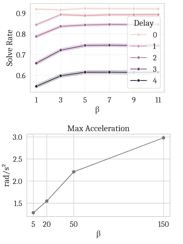
We can’t expect our neural network outputs to be perfect, so $\beta$ is a guidance weight clipping parameter which is used to manage instability, especially when running denoising with a small number of steps (i.e big steps). The RTC work does a sweep on $\beta$, measuring the success rate for the task the robot is meant to be doing, and the maximum acceleration between action chunks (poorer inpainting means sharper discontinuities between chunks, therefore higher acceleration). They find $\beta=5$ to be a happy medium (success rate doesn’t increase above this value, but maximum acceleration does).
In the next section we we will put a magnifying glass on one of the key assumptions that led to deriving equation 3 and show that by adjusting the assumption, we can get even smoother robot policies.
How we got smooth-as-butter robot policies
Without following all of the steps of the derivation in ΠGDM, we can at least discuss one key consideration behind how the guidance weight is derived. In order to consider $p_\tau(\mathbf{Y} \mid \mathbf{A}^\tau)$ from equation 1, it’s necessary to have some assumption on the prior distribution $p_1(\mathbf{A^1})$.
To see why $p_1(\mathbf{A^1})$ is being put in the spotlight, we need to understand how a concrete $\mathbf{A^\tau}$ influences our chances of recovering $\mathbf{Y}$ after denoising. So, given a concrete $\mathbf{A^\tau}$, we can ask ourselves what the distribution of $\mathbf{A^1}$ looks like. That is, we can consider $p_\tau(\mathbf{A^1} \mid \mathbf{A}^\tau)$. And given that distribution, we can ask about the likelihood that our inpainting condition $\mathbf{W} \odot \mathbf{A^1} = \mathbf{Y}$ is satisfied.
Now, By Bayes’ rule
\[\begin{equation}p_\tau(\mathbf{A}^1 \mid \mathbf{A}^\tau) \propto p_1(\mathbf{A}^1) \cdot p_\tau(\mathbf{A}^\tau \mid \mathbf{A}^1)\tag{7}\end{equation}\]Recall that the forward noising process for flow matching is $p_\tau(\mathbf{A^\tau}\mid\mathbf{A^1}) = \mathcal{N}(\tau \mathbf{A^1},(1 - \tau)^2\mathbf{I})$ by construction, no assumptions here. So what’s left is $p_1(\mathbf{A^1})$. Clearly, the assumptions we make about $p_1(\mathbf{A^1})$ play directly into $p_\tau(\mathbf{Y} \mid \mathbf{A}^\tau)$, and ultimately, the correction term in $\mathbf{v_{\Pi \text{GDM}}}$ from equation 3.
ΠGDM (and many other works in related derivations) make the reasonable approximation $p_1(\mathbf{A^1}) = \mathcal{N}(\mathbf{0}, \sigma_d^2\mathbf{I})$ with $\sigma_d^2=1$ (in fact, the $\sigma_d^2$ is often omitted, but we will see soon why I kept it in). Consider an image generation model for example, where we normalize pixels to have mean 0 and standard deviation 1. With a large corpus of images in our training data, a standard normal distribution is the most reasonable assumption we can make while still remaining general.
It then turns out that, with a little bit of work (product of gaussians, change of variables to move to the flow matching formulation), we can derive.
\[\begin{equation} r_\tau^2 = \frac{(1 - \tau)^2 \sigma_d^2}{(1 - \tau)^2 + \sigma_d^2 \tau^2} \tag{8} \end{equation}\]In the RTC paper (and equation 5 above) $\sigma_d$ is not mentioned as it is just assumed to be 1.
But, should we really be assuming $\sigma_d=1$ for action trajectory generation? We need to remind ourselves that for action trajectory generation, we condition on an observation. In fact, we have been omitting this conditioning in the notation above. The prior data distribution should more correctly be written $p_1(\mathbf{A^1}\mid \mathbf{o})$, where $\mathbf{o}$ is the observation. And we should also be more precise and write $\sigma_{d\mid\mathbf{o}}$ in equation 8.
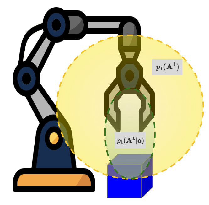
To illustrate why this is important, let’s take an example scenario, where the task is to pick up a blue block, and our robot gripper is above the block. Clearly the only reasonable course of action is to move down towards the block. Considering we had previously collected a large dataset of state-action pairs, and normalized the actions to have mean 0 and standard deviation 1, it’s clear that given the blue block observation, the conditioned prior distribution $p_1(\mathbf{A^1}\mid \mathbf{o})$ (green ellipsoid in the figure below) has a much smaller variance than the full dataset (yellow ellipsoid in the figure below).
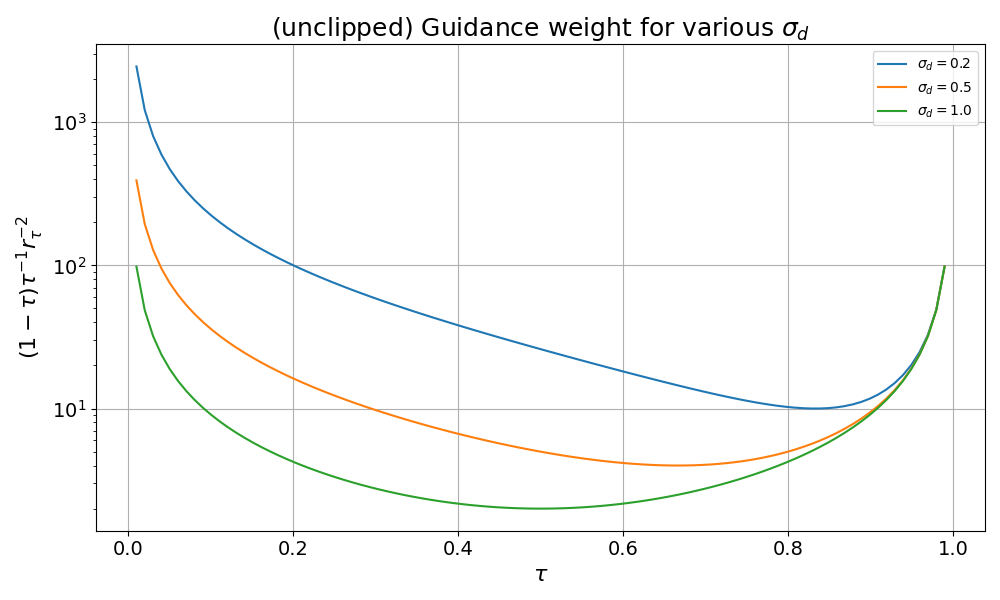
Now we know that $\sigma_{d\mid\mathbf{o}} « 1$. This has non-trivial effect on $r_\tau^2$ as can be seen in equation 8, and ultimately on the correction term of equation 3 where $r_\tau^2$ is on the denominator. It actually results in an increase to the guidance weight (if we ignore the $\beta$ clipping).
Here’s the full guidance weight coefficient $(1-\tau)\tau^{-1}r_\tau^{-2}$, plotted for various values of $\sigma_{d\mid\mathbf{o}}$.
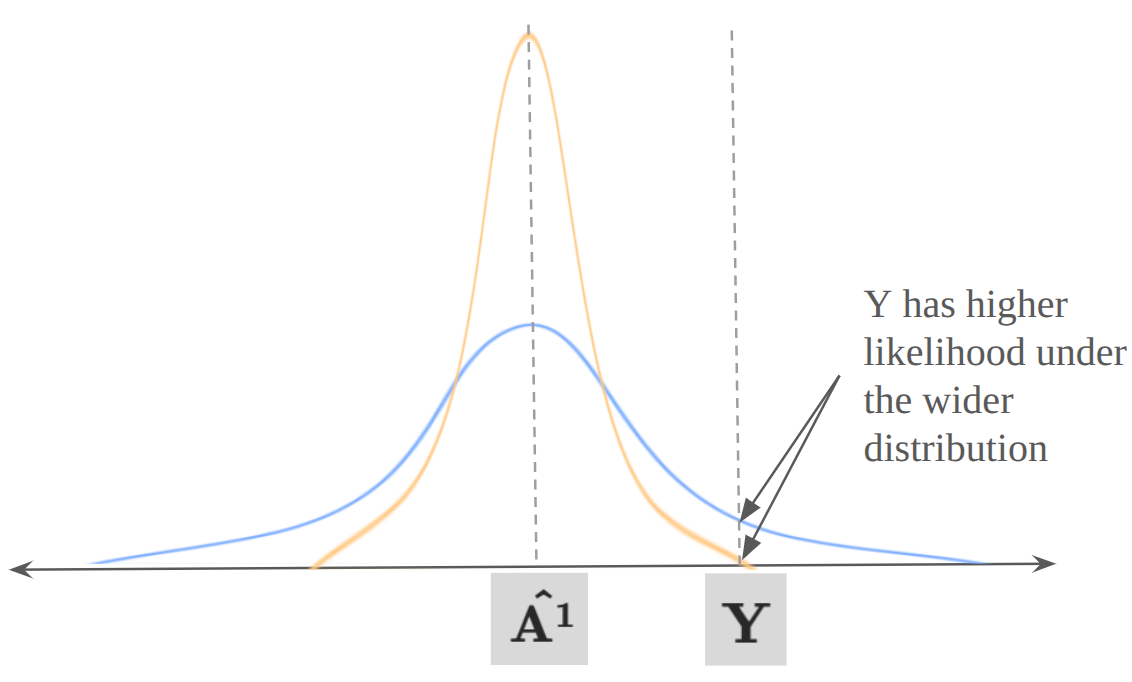
To really hammer in the intuition around why a narrower prior data distribution results in a stronger guidance term, let’s look at the problem from one more angle. Recall that the correction term of equation 3 (shown on its own in equation 6) is the VJP, and this points on the direction of steepest descent of the loss function $\mid\mid\mathbf{Y} - \mathbf{\hat{A^1}}\mid\mid^2$. The figure below shows a 1D representation of the data space, with $\mathbf{Y}$ and $\mathbf{\hat{A^1}}$ fixed at specific values. The gaussian curves represent two versions of what $p_\tau(\mathbf{A^1} \mid \mathbf{A^\tau}, \mathbf{o})$ might look like depending on $r_\tau^2$ (and ultimately $\sigma_{d\mid{\mathbf{o}}}$), and recall from equation 7 that the prior distribution $p_1(\mathbf{A^1}\mid \mathbf{o})$ directly impacts $p_\tau(\mathbf{A^1} \mid \mathbf{A^\tau}, \mathbf{o})$ . Under the wider distribution ( $\sigma_{d\mid\mathbf{o}}=1$, blue on the figure), $\mathbf{Y}$ has a higher likelihood. Under the narrower distribution ( $\sigma_{d\mid\mathbf{o}} « 1$, yellow on the figure), $\mathbf{Y}$ has a lower likelihood, and therefore we must be more aggressive with our steering in order to shift the distribution $p_\tau(\mathbf{A^1} \mid \mathbf{A^\tau}, \mathbf{o})$ of the inpainting objective towards $\mathbf{Y}$.
Deciding exactly what $\sigma_{d\mid\mathbf{o}}$ should be, can be done empirically via a hyperparameter sweep (which will be included below), but one can also reason about an appropriate value by just considering the whole action space, and how much that’s narrowed down when we want to move the end effector in a specific direction.
What about the clipping term $\beta$?
Finally, we need to briefly discuss the guidance weight clipping parameter $\beta$. Recall that this is there to avoid instability when using a small number of denoising steps (i.e larger denoising steps). The RTC work determines 5 to be a good value for this.
We make the observation that, since the denoising update step
\[\begin{equation}\mathbf{A}^{\tau + \frac{1}{n}} = \mathbf{A}^\tau + \frac{1}{n} \, \mathbf{v}_{\Pi \text{GDM}}(\mathbf{A}^\tau, \mathbf{o}, \tau)\tag{9}\end{equation}\]multiplies $\mathbf{v} _ {\Pi {\text{GDM}}}$ by $1/n$ ($n$ being the number of denoising steps), we can safely scale $\beta$ with $n$. We will also see in the results below, that by using a more appropriate $\sigma_{d\mid\mathbf{o}}$, we may be able to get better results by pushing $\beta$ beyond $n$.
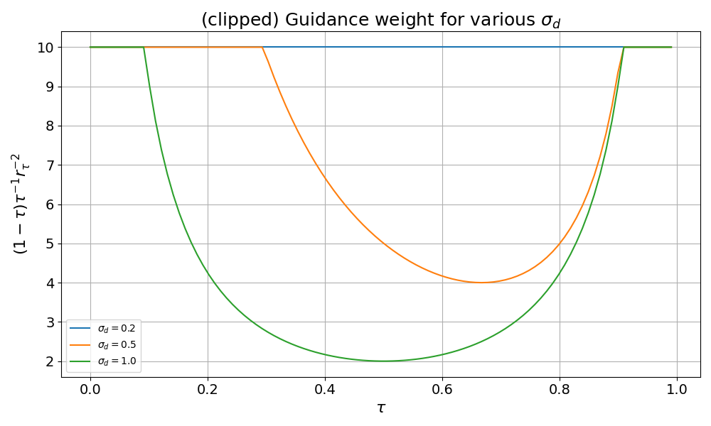
To appreciate the effect of $\beta$, here’s the same plot of guidance scales as above, now clipped with $\beta=10$.
Experiments: what smooth-as-butter robot policies look like
So what do these tweaks translate to with real robots? Well, we fine-tuned π₀ on an ALOHA setup for the task of folding dinner napkins. Then we tried variations based on our two tweaks.
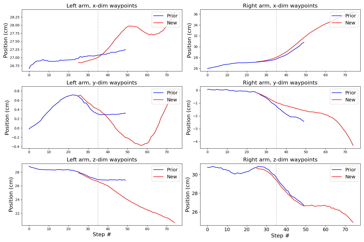
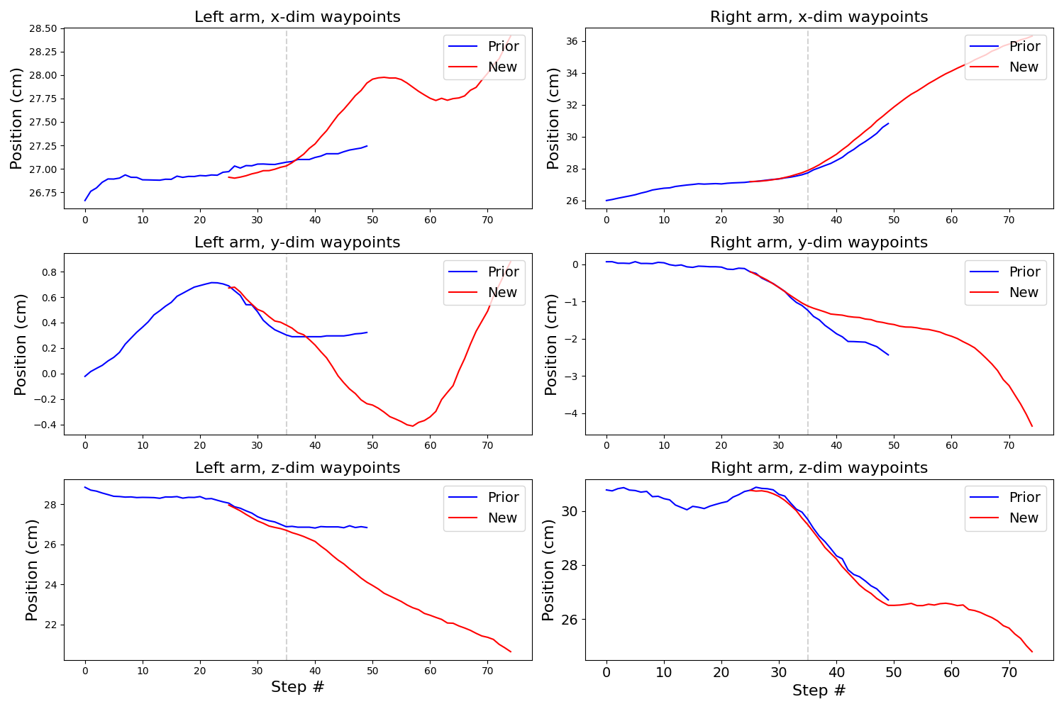
The following plots have two columns. The left column shows action chunks for the left arm, the right column shows action chunks for the right arm. Each row is one cartesian co-ordinate of the task space command (our policy is trained to produce joint targets, and we use forward-kinematics to translate those into task space). The traces are:
- (blue) is an initial action chunk. This is actually a sequence of 50 actions from some pre-recorded demonstration data.
- (red) is the next action chunk, generated based on the observation at step 25, and inpainted with the remainder of the blue chunk from that step and onwards.
- The inference delay is 9 steps. We indicate that with the grey dotted line, which is placed at the 34th step. In a real rollout, this is where we would switch from the blue chunk to the red chunk.
For each plot we will vary the number of flow matching steps $n$, the assumed prior data standard deviation $\sigma_{d\mid\mathbf{o}}$, and the clipping parameter $\beta$.
It’s worth taking the time to check the scales in the y-axes, noting that they are in units of cm. This will give you a good appreciation for how these curves manifest in a real robot rollout.
Baseline with β=5.0 (n=10 σd=1.0 β=5.0)
These are the settings indicated in RTC, although we use 10 flow matching steps, while sticking to $\beta=5$. Notice the gaps formed between the red and blue chunk, along the vertical gray dotted line. These indicate abrupt transitions, which we don’t want.
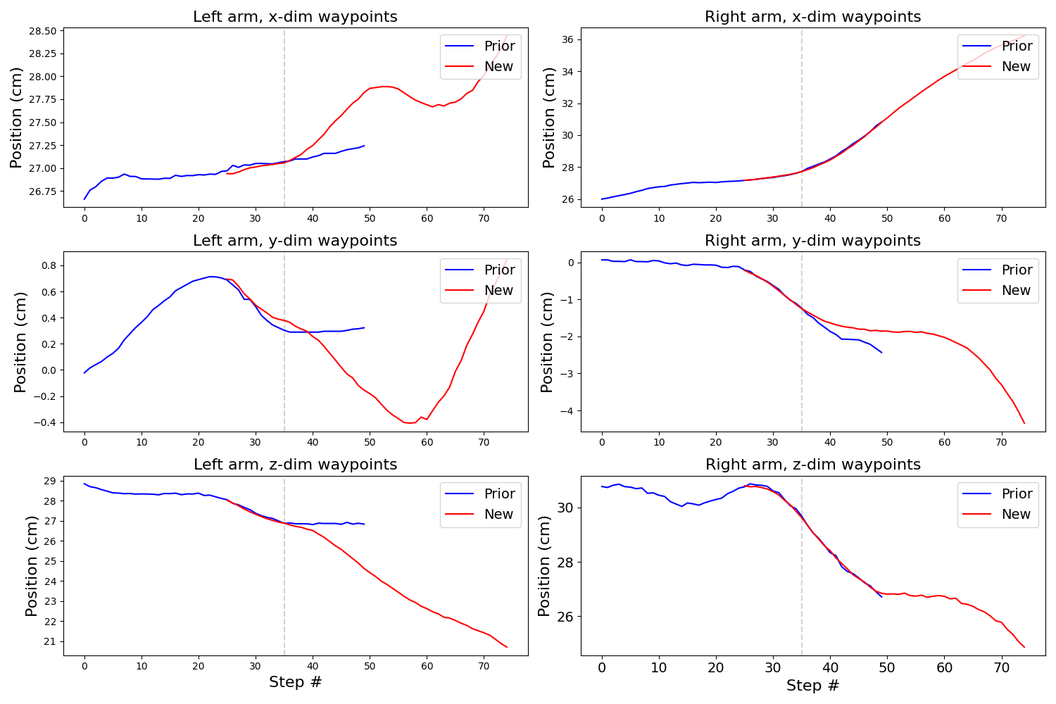
Baseline with β=10.0 (n=10 σd=1.0 β=10.0)
Now we increase $\beta$ to 10 to match $n=10$.
This looks a little better, but there is still room for improvement.
Ours with smaller σd (n=10 σd=0.2 β=10.0)
With our tweaks, things look a lot better! Notice how only one of the plots has an appreciable discrepancy between blue and red at the transition step, and even that is relatively small.
All of the above plots were done with the same starting (blue) chunks. These happen to be from the start of a particular napkin folding demonstration. We can repeat this analysis for many chunks throughout several episodes. For each plot above, we can compute the “discrepancy” for each arm at the transition point as the L2 norm between the commanded task space cartesian co-ordinates (np.linalg.norm(blue_xyz - red_xyz)). Then we can compute the mean and standard deviation over the chunks and arms. The plot below shows just that for the three settings shared above. The settings are shown on the x axis, the centers of the vertical lines are the means, and the heights of the lines extend one standard deviation below and above the centers.
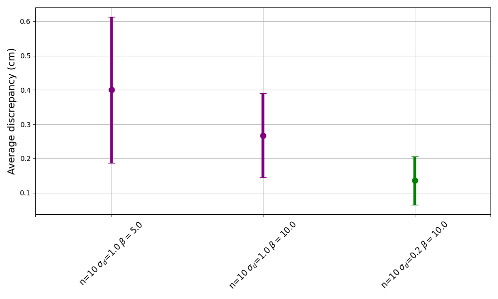
Our setting with n=10 σ=0.2 β=10.0 is clearly an improvement over the baselines.
Note: These are the settings used in the video at the top of this post.
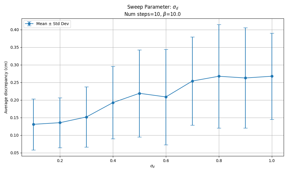
Sweeping $\sigma_{d\mid\mathbf{o}}$
We tried running a sweep over $\sigma_{d\mid\mathbf{o}}$ with our preferred settings for the other parameters. Below we plot the results of the same quantity in the plot above (average of all np.linalg.norm(blue_xyz - red_xyz) at the transition point between chunks, over several episodes). Clearly, reducing $\sigma_{d\mid\mathbf{o}}$ helps. We decided to stick with $\sigma_{d\mid\mathbf{o}}=0.2$ as the results don’t improve much below that.
Sweeping $\beta$
We sweeped $\beta$ for various values of $n$ to check our claim that we can safely scale $\beta$ with $n$. For $n=10$, we see good discrepancy metrics for $\beta \in [10, 16]$. But we need to remember that these results are based on just a few episodes. When we tried this with actual robot rollouts we found it was safer to stick to $\beta=10$, with $\beta=14$ causing erratic robot movements.
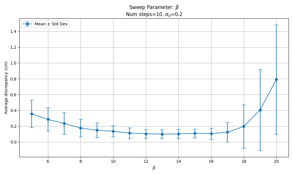
With 20 denoising steps, results indicate good discrepancy metrics for $\beta \in [20, 32]$.
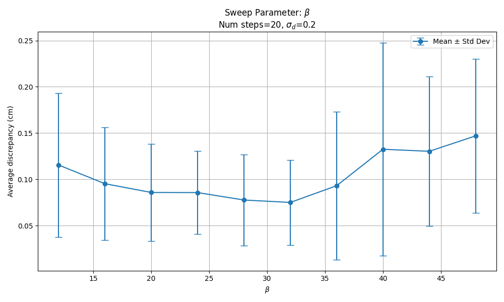
In real robot rollouts we found using $\beta=25$ safely avoided instabilities, but we see no good reason to push beyond $\beta = 20$.
With 5 denoising steps, we see good discrepancy metrics for $\beta \in [5, 8]$.
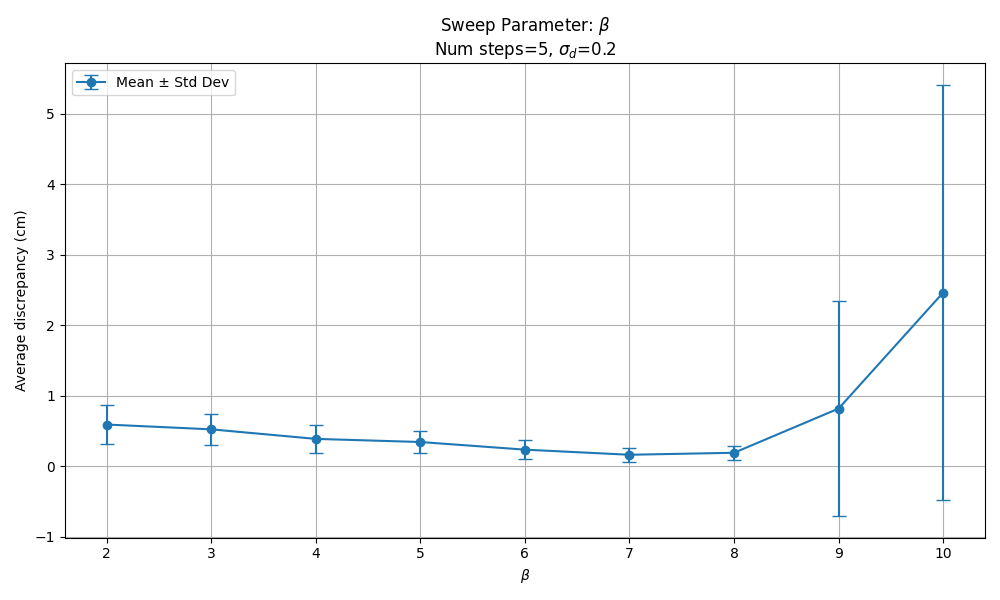
Generally our rule of thumb is to stick with the $\beta=n$ scaling. It removes a hyperparameter, hasn’t failed for us (yet), and there’s little to be gained by trying higher values of $\beta$.
Key takeaway
The key take-away is that a stronger guidance weight is appropriate in action trajectory generation settings where the (conditioned) prior data distribution is narrow. In this blog post, we’ve detailed how to do that in a principled manner, and shown results on a real robot to back it up.
Please feel free to cite this work as
@misc{soare2025smoothrobotpolicies,
  author = {Alexander Soare},
  title = {Smooth-As-Butter Robot Policies},
  year = {2025},
  url = {https://alexander-soare.github.io/robotics/2025/08/05/smooth-as-butter-robot-policies.html},
  note = {Blog post}
}